kaggle-titanic-transcription

Kaggle titanic 필사 정리

import numpy as np
import pandas as pd
import matplotlib.pyplot as plt
import seaborn as sns

plt.style.use('seaborn')
sns.set(font_scale=2.5) 
# matplotlib 의 기본 scheme 말고 seaborn scheme 을 세팅하고, 일일이 graph 의 font size 를 지정할 필요 없이 
#seaborn 의 font_scale 을 사용하면 편합니다.

import plotly.offline as py
py.init_notebook_mode(connected=True)
import plotly.graph_objs as go
import plotly.tools as tls

#ignore warnings
import warnings
warnings.filterwarnings('ignore')

%matplotlib inline

df_train = pd.read_csv('../Study_DA/titanic/train.csv')
df_test = pd.read_csv('../Study_DA/titanic/test.csv')

df_train['FamilySize'] = df_train['SibSp'] + df_train['Parch'] + 1 # 자신을 포함해야하니 1을 더합니다
df_test['FamilySize'] = df_test['SibSp'] + df_test['Parch'] + 1 # 자신을 포함해야하니 1을 더합니다

3.1 Fill Null

null 값을 확인하고 채웁니다.

어떻게 채우는지는 다른 column을 참고하거나 아이디어 혹은 column 평균등으로 대체 가능합니다

for col in df_train.columns:
    msg = 'column: {:>10}\t Percent of NaN value: {:.2f}%'.format(col, 100 * (df_train[col].isnull().sum() / df_train[col].shape[0]))
    print(msg)

column: PassengerId	 Percent of NaN value: 0.00%
column:   Survived	 Percent of NaN value: 0.00%
column:     Pclass	 Percent of NaN value: 0.00%
column:       Name	 Percent of NaN value: 0.00%
column:        Sex	 Percent of NaN value: 0.00%
column:        Age	 Percent of NaN value: 19.87%
column:      SibSp	 Percent of NaN value: 0.00%
column:      Parch	 Percent of NaN value: 0.00%
column:     Ticket	 Percent of NaN value: 0.00%
column:       Fare	 Percent of NaN value: 0.00%
column:      Cabin	 Percent of NaN value: 77.10%
column:   Embarked	 Percent of NaN value: 0.22%
column: FamilySize	 Percent of NaN value: 0.00%

for col in df_test.columns:
    msg = 'column: {:>10}\t Percent of NaN value: {:.2f}%'.format(col, 100 * (df_test[col].isnull().sum() / df_test[col].shape[0]))
    print(msg)

column: PassengerId	 Percent of NaN value: 0.00%
column:     Pclass	 Percent of NaN value: 0.00%
column:       Name	 Percent of NaN value: 0.00%
column:        Sex	 Percent of NaN value: 0.00%
column:        Age	 Percent of NaN value: 20.57%
column:      SibSp	 Percent of NaN value: 0.00%
column:      Parch	 Percent of NaN value: 0.00%
column:     Ticket	 Percent of NaN value: 0.00%
column:       Fare	 Percent of NaN value: 0.24%
column:      Cabin	 Percent of NaN value: 78.23%
column:   Embarked	 Percent of NaN value: 0.00%
column: FamilySize	 Percent of NaN value: 0.00%

Test set에서 Fare 결측값 한개를 찾을 수 있었는데 이는 평균값으로 대체합니다

df_test.loc[df_test.Fare.isnull(), 'Fare']

152   NaN
Name: Fare, dtype: float64

df_test.loc[df_test.Fare.isnull(), 'Fare'] = df_test['Fare'].mean()

df_test['Fare'].mean()

35.6271884892086

df_test.loc[152]

PassengerId                  1044
Pclass                          3
Name           Storey, Mr. Thomas
Sex                          male
Age                          60.5
SibSp                           0
Parch                           0
Ticket                       3701
Fare                      35.6272
Cabin                         NaN
Embarked                        S
FamilySize                      1
Name: 152, dtype: object

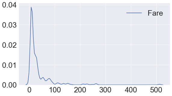
df_train['Fare'].describe()

count    891.000000
mean      32.204208
std       49.693429
min        0.000000
25%        7.910400
50%       14.454200
75%       31.000000
max      512.329200
Name: Fare, dtype: float64

# Fare의 분포를 보고자 plot을 그림 한쪽으로 기울어짐
fig, ax = plt.subplots(1, 1, figsize=(9, 5))
sns.kdeplot(df_train['Fare'], ax=ax)
plt.show()

log_fare = df_train['Fare'].map(lambda i: np.log(i) if i > 0 else 0)

fig, ax = plt.subplots(1, 1, figsize=(9, 5))
sns.kdeplot(log_fare, ax=ax)
plt.show()

왜 log을 취하는 것일까??

복잡한 계산을 쉽게 만들고 왜도와 첨도를 줄여 의미있는 결과 도출하기 위해서!

df_train['Fare'] = df_train['Fare'].map(lambda i: np.log(i) if i > 0 else 0)
df_test['Fare'] = df_test['Fare'].map(lambda i: np.log(i) if i > 0 else 0)

정규표현식?

특정한 규칙을 가진 문자열의 집합을 표현하는 데 사용하는 형식 언어

출처 위키백과

### 영어로 시작하는 문자열중 온점(.)앞에 있는 문자열만 extract해라

df_train['Initial']= df_train.Name.str.extract('([A-Za-z]+)\.') #lets extract the Salutations
    
df_test['Initial']= df_test.Name.str.extract('([A-Za-z]+)\.') #lets extract the Salutations

df_train['Name'].head()

                            Braund, Mr. Owen Harris
  Cumings, Mrs. John Bradley (Florence Briggs Th...
                             Heikkinen, Miss. Laina
       Futrelle, Mrs. Jacques Heath (Lily May Peel)
                           Allen, Mr. William Henry
Name: Name, dtype: object

df_train['Initial'].head()

    Mr
   Mrs
  Miss
   Mrs
    Mr
Name: Initial, dtype: object

pandas 의 crosstab 을 이용하여 우리가 추출한 Initial 과 Sex 간의 count 를 살펴본다

확실히 구분이 가는 것을 볼 수 있다 이를 통해 특정 데이터 값을 원하는 값으로 치환을 해준다

pd.crosstab(df_train['Initial'], df_train['Sex']).T.style.background_gradient(cmap='summer_r') #Checking the Initials with the Sex

Initial	Capt	Col	Countess	Don	Dr	Jonkheer	Lady	Major	Master	Miss	Mlle	Mme	Mr	Mrs	Ms	Rev	Sir
Sex
female	0	0	1	0	1	0	1	0	0	182	2	1	0	125	1	0	0
male	1	2	0	1	6	1	0	2	40	0	0	0	517	0	0	6	1

df_train['Initial'].replace(['Mlle','Mme','Ms','Dr','Major','Lady','Countess','Jonkheer','Col','Rev','Capt','Sir','Don', 'Dona'],
                        ['Miss','Miss','Miss','Mr','Mr','Mrs','Mrs','Other','Other','Other','Mr','Mr','Mr', 'Mr'],inplace=True)

df_test['Initial'].replace(['Mlle','Mme','Ms','Dr','Major','Lady','Countess','Jonkheer','Col','Rev','Capt','Sir','Don', 'Dona'],
                        ['Miss','Miss','Miss','Mr','Mr','Mrs','Mrs','Other','Other','Other','Mr','Mr','Mr', 'Mr'],inplace=True)

df_train.groupby('Initial')['Age'].describe()

	count	mean	std	min	25%	50%	75%	max
Initial
Master	36.0	4.574167	3.619872	0.42	1.000	3.5	8.0	12.0
Miss	150.0	21.860000	12.828485	0.75	14.625	21.5	30.0	63.0
Mr	409.0	32.739609	12.875632	11.00	23.000	30.0	40.0	80.0
Mrs	110.0	35.981818	11.390469	14.00	28.000	35.0	44.0	63.0
Other	9.0	45.888889	12.604012	27.00	38.000	51.0	56.0	60.0

df_train.groupby('Initial').mean()

	PassengerId	Survived	Pclass	Age	SibSp	Parch	Fare	FamilySize
Initial
Master	414.975000	0.575000	2.625000	4.574167	2.300000	1.375000	3.340710	4.675000
Miss	411.741935	0.704301	2.284946	21.860000	0.698925	0.537634	3.123713	2.236559
Mr	455.880907	0.162571	2.381853	32.739609	0.293006	0.151229	2.651507	1.444234
Mrs	456.393701	0.795276	1.984252	35.981818	0.692913	0.818898	3.443751	2.511811
Other	564.444444	0.111111	1.666667	45.888889	0.111111	0.111111	2.641605	1.222222

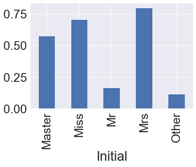
miss,mrs가 높은 것을 확인 할 수 있었다.

df_train.groupby('Initial')['Survived'].mean().plot.bar()

<matplotlib.axes._subplots.AxesSubplot at 0x24c40f5c5c0>

df_train.groupby('Initial').mean()

	PassengerId	Survived	Pclass	Age	SibSp	Parch	Fare	FamilySize
Initial
Master	414.975000	0.575000	2.625000	4.574167	2.300000	1.375000	3.340710	4.675000
Miss	411.741935	0.704301	2.284946	21.860000	0.698925	0.537634	3.123713	2.236559
Mr	455.880907	0.162571	2.381853	32.739609	0.293006	0.151229	2.651507	1.444234
Mrs	456.393701	0.795276	1.984252	35.981818	0.692913	0.818898	3.443751	2.511811
Other	564.444444	0.111111	1.666667	45.888889	0.111111	0.111111	2.641605	1.222222

Age의 결측값을 채우기위해 initial 데이터를 활용합니다. 위의 나와있는 것처럼 intial 별 Age의 평균값으로 대체해줍니다.

df_train.loc[(df_train.Age.isnull())&(df_train.Initial=='Mr'),'Age'] = 33
df_train.loc[(df_train.Age.isnull())&(df_train.Initial=='Mrs'),'Age'] = 36
df_train.loc[(df_train.Age.isnull())&(df_train.Initial=='Master'),'Age'] = 5
df_train.loc[(df_train.Age.isnull())&(df_train.Initial=='Miss'),'Age'] = 22
df_train.loc[(df_train.Age.isnull())&(df_train.Initial=='Other'),'Age'] = 46

df_test.loc[(df_test.Age.isnull())&(df_test.Initial=='Mr'),'Age'] = 33
df_test.loc[(df_test.Age.isnull())&(df_test.Initial=='Mrs'),'Age'] = 36
df_test.loc[(df_test.Age.isnull())&(df_test.Initial=='Master'),'Age'] = 5
df_test.loc[(df_test.Age.isnull())&(df_test.Initial=='Miss'),'Age'] = 22
df_test.loc[(df_test.Age.isnull())&(df_test.Initial=='Other'),'Age'] = 46

df_train['Age'].isnull().sum()

df_test['Age'].isnull().sum()

Embarked는 2개의 null 값이 있는데 가장 많은 값을 가지고 있는 S로 채웁니다.

dataframe 의 fillna method 를 이용하면 쉽게 채울 수 있습니다. 여기서 inplace=True 로 하면 df_train 에 fillna 를 실제로 적용하게 됩니다

print('Embarked has ', sum(df_train['Embarked'].isnull()), ' Null values')

Embarked has  2  Null values

df_train['Embarked'].fillna('S', inplace=True)

수치화시킨 카테고리 데이터를 그대로 넣어도 되지만, 모델의 성능을 높이기 위해 one-hot encoding을 해줄 수 있습니다

pd.get_dummies(df_train['Initial']).head()

	Miss	Mr	Mrs
0	0	1	0
1	0	0	1
2	1	0	0
3	0	0	1
4	0	1	0

dummy 변수들을 만들어주고 변수명을 intial을 앞에 써준다 대신 원래 변수는 제거해준다

df_train= pd.get_dummies(df_train,prefix='Initial',drop_first=True)
df_train.head()

	PassengerId	Survived	Pclass	Age	SibSp	Fare	FamilySize	...	Initial_S	Initial_Miss	Initial_Mr	Initial_Mrs
0	1	0	3	22.0	1	1.981001	2	...	1	0	1	0
1	2	1	1	38.0	1	4.266662	2	...	0	0	0	1
2	3	1	3	26.0	0	2.070022	1	...	1	1	0	0
3	4	1	1	35.0	1	3.972177	2	...	1	0	0	1
4	5	0	3	35.0	0	2.085672	1	...	1	0	1	0

5 rows × 1731 columns

df_test = pd.get_dummies(df_test, columns=['Initial'], prefix='Initial')

#df_train['Initial'] - 에러 발생하는 것을 확인할 수 있다

kaggle-titanic-transcription

Kaggle titanic 필사 정리

3.1 Fill Null

null 값을 확인하고 채웁니다.

어떻게 채우는지는 다른 column을 참고하거나 아이디어 혹은 column 평균등으로 대체 가능합니다

Test set에서 Fare 결측값 한개를 찾을 수 있었는데 이는 평균값으로 대체합니다

왜 log을 취하는 것일까??

복잡한 계산을 쉽게 만들고 왜도와 첨도를 줄여 의미있는 결과 도출하기 위해서!

정규표현식?

특정한 규칙을 가진 문자열의 집합을 표현하는 데 사용하는 형식 언어

출처 위키백과

pandas 의 crosstab 을 이용하여 우리가 추출한 Initial 과 Sex 간의 count 를 살펴본다

확실히 구분이 가는 것을 볼 수 있다 이를 통해 특정 데이터 값을 원하는 값으로 치환을 해준다

miss,mrs가 높은 것을 확인 할 수 있었다.

Age의 결측값을 채우기위해 initial 데이터를 활용합니다. 위의 나와있는 것처럼 intial 별 Age의 평균값으로 대체해줍니다.

Embarked는 2개의 null 값이 있는데 가장 많은 값을 가지고 있는 S로 채웁니다.

dataframe 의 fillna method 를 이용하면 쉽게 채울 수 있습니다. 여기서 inplace=True 로 하면 df_train 에 fillna 를 실제로 적용하게 됩니다

수치화시킨 카테고리 데이터를 그대로 넣어도 되지만, 모델의 성능을 높이기 위해 one-hot encoding을 해줄 수 있습니다

dummy 변수들을 만들어주고 변수명을 intial을 앞에 써준다 대신 원래 변수는 제거해준다

참고

kaggle kr(https://kaggle-kr.tistory.com/18)

위키백과(https://ko.wikipedia.org/wiki/%EC%A0%95%EA%B7%9C_%ED%91%9C%ED%98%84%EC%8B%9D)

gangsss.github.io

Kaggle titanic 필사 정리

3.1 Fill Null

null 값을 확인하고 채웁니다.

어떻게 채우는지는 다른 column을 참고하거나 아이디어 혹은 column 평균등으로 대체 가능합니다

Test set에서 Fare 결측값 한개를 찾을 수 있었는데 이는 평균값으로 대체합니다

왜 log을 취하는 것일까??

복잡한 계산을 쉽게 만들고 왜도와 첨도를 줄여 의미있는 결과 도출하기 위해서!

정규표현식?

특정한 규칙을 가진 문자열의 집합을 표현하는 데 사용하는 형식 언어

출처 위키백과

pandas 의 crosstab 을 이용하여 우리가 추출한 Initial 과 Sex 간의 count 를 살펴본다

확실히 구분이 가는 것을 볼 수 있다 이를 통해 특정 데이터 값을 원하는 값으로 치환을 해준다

miss,mrs가 높은 것을 확인 할 수 있었다.

Age의 결측값을 채우기위해 initial 데이터를 활용합니다. 위의 나와있는 것처럼 intial 별 Age의 평균값으로 대체해줍니다.

Embarked는 2개의 null 값이 있는데 가장 많은 값을 가지고 있는 S로 채웁니다.

dataframe 의 fillna method 를 이용하면 쉽게 채울 수 있습니다. 여기서 inplace=True 로 하면 df_train 에 fillna 를 실제로 적용하게 됩니다

수치화시킨 카테고리 데이터를 그대로 넣어도 되지만, 모델의 성능을 높이기 위해 one-hot encoding을 해줄 수 있습니다

dummy 변수들을 만들어주고 변수명을 intial을 앞에 써준다 대신 원래 변수는 제거해준다

참고

kaggle kr(https://kaggle-kr.tistory.com/18)

위키백과(https://ko.wikipedia.org/wiki/%EC%A0%95%EA%B7%9C_%ED%91%9C%ED%98%84%EC%8B%9D)

Share this post